Infill vs. boundary expansion: telling them apart in satellite imagery
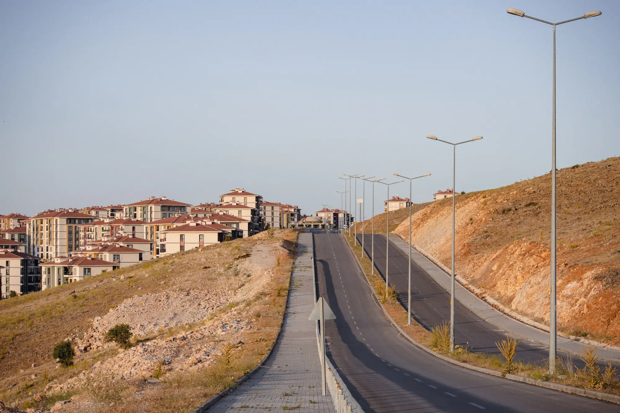
A new cluster of rooftops shows up on this year's imagery. Before you log it as anything, you need to answer one question: is this infill, or did the city step over the line? The two look similar from above at first glance. A block of new roofs is a block of new roofs. But they mean very different things for a growth management report, and they read differently once you know what to look for.
What separates infill from boundary expansion
Infill is new construction inside the approved urban footprint, usually on vacant lots, underused parcels, or land between existing streets that never got built out. It's growth the plan already accounted for. Boundary expansion is new built-up area outside the line, on land that was zoned agricultural, conservation, or simply not yet opened for development. One is the plan working as intended. The other is the thing a growth boundary exists to catch.
On the ground these two produce different footprints. Infill tends to fill gaps: a parcel here, a cul-de-sac there, slotted into a street grid that already exists on both sides. Boundary expansion tends to show up as a new cluster with its own internal road pattern, often following a ridge, a frontage road, or a field boundary that has nothing to do with the city's existing grid. It's new, not patched in.
Reading the signal in medium-resolution imagery
At 3 to 10 meter resolution, you're not counting individual houses, you're reading built-up texture: pixel clusters that shift from bare soil or vegetation to impervious surface and roofline. A few things tend to separate the two patterns once you're looking at change layers year over year rather than a single scene.
Infill shows up as isolated pixels or small clusters surrounded on most sides by built-up pixels from the prior year. The new signal sits inside an already-built matrix. Boundary expansion shows up as a contiguous patch of new built-up pixels that borders undeveloped land on one or more sides, and critically, sits on the far side of the boundary vector when you overlay it.
That overlay step is the part that settles the question. Imagery alone won't tell you which side of the line a parcel falls on; you need the approved boundary as a georeferenced layer, laid directly on top of the built-up change detection. Pixels that light up inside the polygon are infill by definition, regardless of how dense or sparse the surrounding fabric is. Pixels that light up outside it are expansion, full stop, even if they're adjacent to the line and look modest on the ground.
A simple classification that holds up in a report
Once you have both layers, that is, this year's built-up change and the boundary polygon, the classification itself is just a spatial join. Every new built-up pixel gets tagged inside or outside. Sum the outside pixels, convert to hectares, and you have the figure a planning commission needs: how many hectares of this year's expansion fell where the plan didn't call for it.
The harder part has historically been getting the two layers lined up and checked on a reliable schedule, rather than reconstructing it after the fact from old aerial photos and a stack of permit records. That's the gap Urban Growth Monitor is built to close: an annual built-up footprint laid against the approved boundary, with the outside-the-line hectares called out as a standalone figure rather than buried in a narrative.
If you're staring at a change map right now trying to decide which side of the line a new cluster falls on, that's the question this tool is built to answer, year after year.